Файл:MUSIC MVDR.png
Перейти до навігації
Перейти до пошуку

Розмір при попередньому перегляді: 800 × 386 пікселів. Інші роздільності: 320 × 154 пікселів | 640 × 309 пікселів | 1342 × 647 пікселів.
Повна роздільність (1342 × 647 пікселів, розмір файлу: 112 КБ, MIME-тип: image/png)
| Відомості про цей файл містяться на Вікісховищі — централізованому сховищі вільних файлів мультимедіа для використання у проектах Фонду Вікімедіа. |
Опис файлу
| Опис |
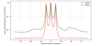
English: Spatial frequencies estimation (source code).
Русский: Оценка пространтвенных частот (исходный код). |
| Час створення | |
| Джерело | Власна робота |
| Автор | Kirlf |
| PNG розвиток | Це PNG графічне зображення було створено з допомогою Matplotlib |
| Сирцевий код | Python code"""
Developed by Vladimir Fadeev
(https://github.com/kirlf)
Kazan, 2017 / 2020
Python 3.7
"""
import numpy as np
import matplotlib.pyplot as plt
"""
Received signal model:
X = A*S + W
where
A = [a(theta_1) a(theta_2) ... a(theta_d)]
is the matrix of steering vectors
(dimension is M x d,
M is the number of sensors,
d is the number of signal sources),
A steering vector represents the set of phase delays
a plane wave experiences, evaluated at a set of array elements (antennas).
The phases are specified with respect to an arbitrary origin.
theta is Direction of Arrival (DoA),
S = 1/sqrt(2) * (X + iY)
is the transmit (modulation) symbols matrix
(dimension is d x T,
T is the number of snapshots)
(X + iY) is the complex values of the signal envelope,
W = sqrt(N0/2)*(G1 + jG2)
is additive noise matrix (AWGN)
(dimension is M x T),
N0 is the noise spectral density,
G1 and G2 are the random Gaussian distributed values.
"""
M = 10 # number of sensors
SNR = 10 # Signal-to-Noise ratio (dB)
d = 3 # number sources of EM waves
N = 50 # number of snapshots
""" Signal matrix """
S = ( np.sign(np.random.randn(d,N)) + 1j * np.sign(np.random.randn(d,N)) ) / np.sqrt(2) # QPSK
""" Noise matrix
Common formula:
AWGN = sqrt(N0/2)*(G1 + jG2),
where G1 and G2 - independent Gaussian processes.
Since Es(symbol energy) for QPSK is 1 W, noise spectral density:
N0 = (Es/N)^(-1) = SNR^(-1) [W] (let SNR = Es/N0);
or in logarithmic scale::
SNR_dB = 10log10(SNR) -> N0_dB = -10log10(SNR) = -SNR_dB [dB];
We have SNR in logarithmic (in dBs), convert to linear:
SNR = 10^(SNR_dB/10) -> sqrt(N0) = (10^(-SNR_dB/10))^(1/2) = 10^(-SNR_dB/20)
"""
W = ( np.random.randn(M,N) + 1j * np.random.randn(M,N) ) / np.sqrt(2) * 10**(-SNR/20) # AWGN
mu_R = 2*np.pi / M # standard beam width
resolution_cases = ((-1., 0, 1.), (-0.5, 0, 0.5), (-0.3, 0, 0.3)) # resolutions
for idxm, c in enumerate(resolution_cases):
""" DoA (spatial frequencies) """
mu_1 = c[0]*mu_R
mu_2 = c[1]*mu_R
mu_3 = c[2]*mu_R
""" Steering vectors """
a_1 = np.exp(1j*mu_1*np.arange(M))
a_2 = np.exp(1j*mu_2*np.arange(M))
a_3 = np.exp(1j*mu_3*np.arange(M))
A = (np.array([a_1, a_2, a_3])).T # steering matrix
""" Received signal """
X = np.dot(A,S) + W
""" Rxx """
R = np.dot(X,np.matrix(X).H)
U, Sigma, Vh = np.linalg.svd(X, full_matrices=True)
U_0 = U[:,d:] # noise sub-space
thetas = np.arange(-90,91)*(np.pi/180) # azimuths
mus = np.pi*np.sin(thetas) # spatial frequencies
a = np.empty((M, len(thetas)), dtype = complex)
for idx, mu in enumerate(mus):
a[:,idx] = np.exp(1j*mu*np.arange(M))
# MVDR:
S_MVDR = np.empty(len(thetas), dtype = complex)
for idx in range(np.shape(a)[1]):
a_idx = (a[:, idx]).reshape((M, 1))
S_MVDR[idx] = 1 / (np.dot(np.matrix(a_idx).H, np.dot(np.linalg.pinv(R),a_idx)))
# MUSIC:
S_MUSIC = np.empty(len(thetas), dtype = complex)
for idx in range(np.shape(a)[1]):
a_idx = (a[:, idx]).reshape((M, 1))
S_MUSIC[idx] = np.dot(np.matrix(a_idx).H,a_idx)\
/ (np.dot(np.matrix(a_idx).H, np.dot(U_0,np.dot(np.matrix(U_0).H,a_idx))))
plt.subplots(figsize=(10, 5), dpi=150)
plt.semilogy(thetas*(180/np.pi), np.real( (S_MVDR / max(S_MVDR))), color='green', label='MVDR')
plt.semilogy(thetas*(180/np.pi), np.real((S_MUSIC/ max(S_MUSIC))), color='red', label='MUSIC')
plt.grid(color='r', linestyle='-', linewidth=0.2)
plt.xlabel('Azimuth angles (degrees)')
plt.ylabel('Power (pseudo)spectrum (normalized)')
plt.legend()
plt.title('Case #'+str(idxm+1))
plt.show()
""" References
1. Haykin, Simon, and KJ Ray Liu. Handbook on array processing and sensor networks. Vol. 63. John Wiley & Sons, 2010. pp. 102-107
2. Hayes M. H. Statistical digital signal processing and modeling. – John Wiley & Sons, 2009.
3. Haykin, Simon S. Adaptive filter theory. Pearson Education India, 2008. pp. 422-427
4. Richmond, Christ D. "Capon algorithm mean-squared error threshold SNR prediction and probability of resolution." IEEE Transactions on Signal Processing 53.8 (2005): 2748-2764.
5. S. K. P. Gupta, MUSIC and improved MUSIC algorithm to esimate dorection of arrival, IEEE, 2015.
"""
|
Ліцензування
Я, власник авторських прав на цей твір, добровільно публікую його на умовах такої ліцензії:
Цей файл ліцензований на умовах Creative Commons Із зазначенням автора - Розповсюдження на тих самих умовах 4.0 Міжнародна
- Ви можете вільно:
- ділитися – копіювати, поширювати і передавати твір
- модифікувати – переробляти твір
- При дотриманні таких умов:
- зазначення авторства – Ви повинні вказати авторство, надати посилання на ліцензію і вказати, чи якісь зміни було внесено до оригінального твору. Ви можете зробити це в будь-який розсудливий спосіб, але так, щоб він жодним чином не натякав на те, наче ліцензіар підтримує Вас чи Ваш спосіб використання твору.
- поширення на тих же умовах – Якщо ви змінюєте, перетворюєте або створюєте іншу похідну роботу на основі цього твору, ви можете поширювати отриманий у результаті твір тільки на умовах такої ж або сумісної ліцензії.
Історія файлу
Клацніть на дату/час, щоб переглянути, як тоді виглядав файл.
| Дата/час | Мініатюра | Розмір об'єкта | Користувач | Коментар | |
|---|---|---|---|---|---|
| поточний | 05:41, 18 лютого 2019 | | 1342 × 647 (112 КБ) | Kirlf | User created page with UploadWizard |
Використання файлу
Така сторінка використовує цей файл:
Глобальне використання файлу
Цей файл використовують такі інші вікі:
- Використання в ca.wikipedia.org
- Використання в en.wikipedia.org
- Використання в ru.wikipedia.org